Behind the Scenes of A/B Testing Recommendation Systems

Take it from the experts. For the more curious amongst you, our scientists provide further details about A/B testing personalization engines against each other. Ready? Then roll up your sleeves and let’s get into the thick of it.

Selecting Key Metrics

It’s essential that the participating vendors of personalization solutions and the client agree on the measurement method and the key performance indicators (KPIs) of the A/B test.  

Primarily, measuring a recommendations solution’s effectiveness should focus on the return on investment (ROI) because choosing the right vendor is, above all, a business decision. We can measure the ROI of the tested recommendation solutions by calculating the cost of implementing them against the added value they generate.

Furthermore, the selected KPIs of an A/B test largely depend on the industry or the business model of the client wishing to compare personalization solutions. From retail through publishing to media streaming, every major online business type has particular aspects that can be enhanced through personalization. 

For instance, in e-commerce, A/B tests of competing personalization engines can measure

• gross merchandising value (GMV), that is, the value of conversions generated by personalized recommendations; 
• this same value compared to the number of recommendations displayed (for instance, GMV/1000 recommendations) 
• click-through rate (CTR), the number of clicks on product recommendations, compared to the number of recommendations displayed.

In the news and publishing sector, typical KPIs of A/B testing recommendation systems include

• number of article pages viewed from recommendations;
• this metric normalized by the number of users receiving the recommendations and calculated within a specific period (usually the duration of the A/B test); or
• conversion into views (long-term CTR) – the number of recommendations resulting in content views divided by the number of recommendation requests. We consider a piece of content viewed if the user has seen at least 10 percent of its length – this aims to exclude clickbait-type content and unintentional clicks. 

In the media streaming industry, A/B tests comparing personalization engines usually measure

• watch time through recommendation – time spent watching videos as a result of recommendations, within a certain timeframe (24 hours after clicking on the recommendation widget) 
• conversion into sales – put simply, the revenue from pay-per-view, and
• time spent on site. 

These are just a handful of options for measuring the impact of personalization in various fields. We’ve compiled the complete list of possible KPIs and their definitions here.

External Factors to Consider

The results of the A/B test may be distorted by a variety of external factors, such as:

• Market effects – for instance, an unforeseen drop in demand for a certain product or service due to industry disruption, like the way Airbnb disrupted the flat rental market in its heyday. 
• Business decisions, for instance, when a mobile payment provider is not supported by certain browsers.
• Marketing campaigns that boost traffic to certain pages of a site for a limited period.
• Seasonal specificities, like a sudden spike in demand for men’s gifts around Fathers’ Day, 
• and other unknown factors. 

These external, potentially variable – or, to use a statistical term, non-stationary factors, also including the day of the week, user device, and the distribution of the visitors should impact the tested solutions in the same way. Therefore, setting up the A/B-test correctly is crucial in order to avoid misleading consequences.

A/A Testing to Validate User Split

Before we take a more detailed look at A/A testing, it’s important to note a difference in scenarios. In the case of A/B testing various digital assets like landing pages or CTA buttons, the A/A test serves to check if the system is working properly. If the A/A test yields different results for the two identical user groups in the test, that signals a problem with the testing mechanism. However, in the case of A/B testing recommendation systems, the A/A test is deployed to make sure that the division of user groups is reliably randomized. 

To perform a theoretically well-justified A/B-test, we have to ensure that the control group and the test group are identical. That is to say, they have no difference in their behavior, in the statistical sense, related to the measurements analyzed in the A/B test. By pure chance, there could be a significant difference between the two groups regarding the tested metric. This would create a bias in the outcome of the A/B test, ultimately rendering the results questionable. A/A tests are conducted to prevent this scenario, in other words, to validate the division of the user groups.

In fact, there are two options for validating the user split: 

• By looking at historical data in respect to the selected KPI, typically from a sufficiently long, recent period, to see if it has statistically equal distribution over the two groups. For instance, if average spending has been significantly higher in one group than in the other, that’s going to skew the results of an A/B test with a spending-related KPI like gross merchandising value. 
• If no reliable historical data are available, that calls for an A/A test. In contrast to A/B testing, this time, both the control and the test group receive the same treatment. In the case of testing personalization engines, both groups receive recommendations from the same personalization solution. Then we measure if there is a statistically significant difference in the selected KPI between the two groups. If there isn’t, that means the users in the two groups behave statistically equally, and no bias can be expected in the A/B test. 
  

Understanding Statistical Significance

During an A/B test, only a sample of users are exposed to the service of each personalization solution. The goal is to determine if the measured difference in their reactions would be valid for all users. For this reason, it is not enough to look at the basic difference between the measurements, that is, the results of the A/B test. It’s also necessary to conduct so-called statistical testing to specify the probability of these results being the same outside the test’s scope.

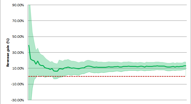
Cumulative revenue gain in percentage and its change over time; the graph shows that the gain is statistically significant because the lower bound of the confidence interval is above zero by the end of the tested period.

The measured difference is considered statistically significant if there is less than a five-percent chance that it’s due to random factors and not caused by the real performance gap between control and test versions. This percentage is referred to as the p value. If it’s less than 0.1 percent, that falls into the category of very strong significance.

If you want to try your hand at gauging the statistical significance of an A/B test, there are a wealth of online tools that do just this.

T-Tests Explained

T-tests are our tools for determining if the difference detected between two variants compared in an A/B test is statistically significant.

Independent two-sample T-tests are used to measure if two sets of data are statistically different from each other. They come in handy when we compare the daily values of the metric observed in the two groups, for example, the additional daily GMV through recommendations, or daily CTR values.

A T-test assumes that (1) the underlying distribution is the normal distribution, and (2) that the two underlying distributions have the same variance. 

Put simply, normal distribution is a natural phenomenon where measurements of a group cluster around the average value. For instance, if we look at the height of children in a class, most of the kids will be around average size, while outliers – those who are shorter or taller than average – will be relatively few. The more measurements we have, the more the data converge towards this normal distribution. If we measure the height of an entire country’s population, this average-vs-outliers pattern will be even more obvious.

As for variance: this metric indicates how far a set of measurements is spread out from their average value. Sticking to the example of the height of a country’s residents: if 90 percent fall into the average height category, their variance is different from another country’s population where only 50 percent are of average height, with more people on both the short and the tall end of the spectrum. And yet, the distribution of each group is normal.

Back to the T-test: first, we have to check if these assumptions are valid.
Pearson’s test checks if the data overturn the assumption of normal distribution. Levene’s test aims to validate the equality of variances in the data.

If the assumption of normal distribution is overturned by the p values of Pearson’s normality test, then the Mann–Whitney U-test should be used instead of the T-test. In other words, the T-test should be executed only if both data sets’ p values are over the standard statistical significance limit, meaning that the probability of the underlying distribution being normal is higher than 95 percent. 

If Levene’s test overturns the assumption of equal variances, then Welch’s T-test is to be used.

The key takeaway is: all these tests serve to determine whether two independent samples were selected from populations having the same distribution.

A Brief Look at Confidence Intervals

Besides statistical significance, which shows the existence of a significant difference in the mean values of two tested personalization solutions, we can also look at the extent of the difference between them. This can be evaluated through confidence intervals. The mean values of a series of measurements can be calculated in various ways. Here we consider micro-and macro-averaging. Macro-averaging computes the given metric for each day during the A/B test and then takes the average of these values. Therefore, it treats all days equally. On the other hand, micro-averaging considers all contributions of the entire A/B testing period and calculates an average value from these.

Only micro-averaged results can be used as a base for establishing confidence intervals. In the case of macro-averaging, the variance in the data has already been accounted for by means of “flattening” the daily values into an average. 

In descriptive statistics, confidence intervals reported along with the mean measurement estimates of the metric concerned indicate the reliability of these estimates. The 95-percent confidence level is commonly used as a benchmark. It can be interpreted as a range of values among which the mean of the population – that’s all possible users, not just the ones that have participated in the A/B-test – can be found with 95-percent certainty.

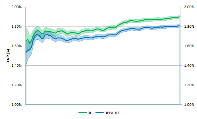
 In this graph comparing the conversion rates (CVR) of two algorithms, the colored fields indicate confidence intervals.

Summary

In this piece, we shed light on some of the finer aspects of A/B testing recommendation systems. We listed some possible KPIs; we looked at the role of external factors and how to make sure they don’t distort our results. We explained why A/A tests often precede A/B tests. We introduced the concept of statistical significance and browsed its arsenal of T-tests. If you didn’t get hooked on statistics by this point, our brief overview of confidence intervals surely did the trick…

On a more serious note: if this material helped you get a clearer picture of A/B testing personalization engines and how it fits into your organization’s roadmap, don’t hesitate to get in touch with us.